You should never use countif function (google spreadsheet)

Sang

Oct 6, 2019 • 2 min read

Recently, I was asked to build a shopping order system for my sister.

Due to the complexity and ambitiousness of the requirement, I initially chose the google spreadsheet to build a simple system before starting with a web-based system.

Then I got to a case that I need to make a cell validation, which ensures there is no ID duplicated in a particular column.

Failed solution

This stack exchange question appeared first when I googled.
Based on the accepted answer, I got the first solution by using the countif function. It works with the following expressions.

  | A    | B |        C
---------------------------------
1 | bar  | 2 | =COUNTIF(A1,A1:A3)
2 | baar | 1 | =COUNTIF(A2,A1:A3)
3 | bar  | 2 | =COUNTIF(A3,A1:A3)
---------------------------------

Column C displays the expressions used in column B

The solution works perfectly until my sister told me that the validation continuously fails even when no duplicated ID entered.

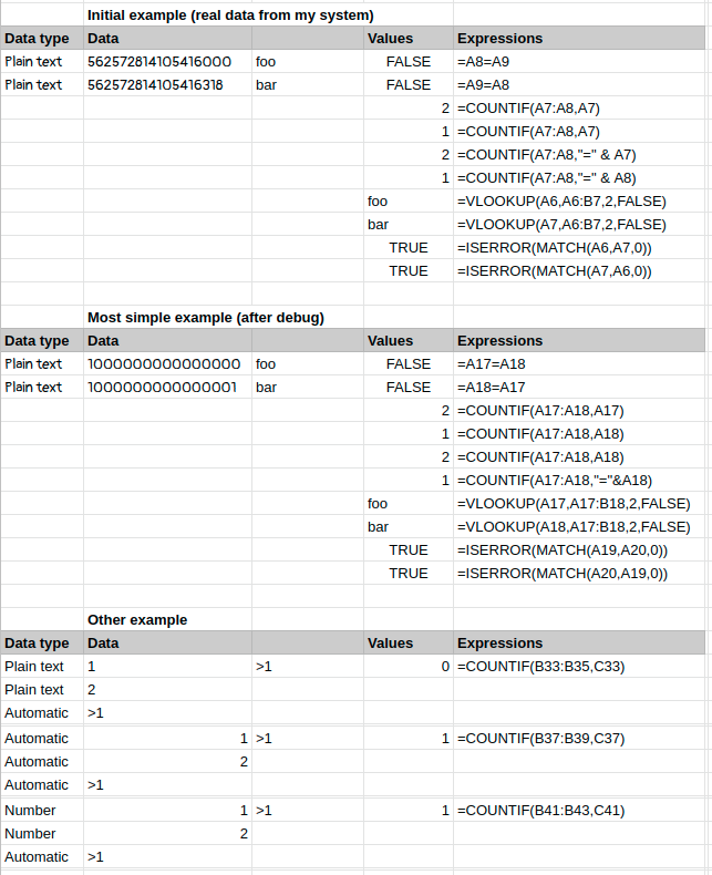
After debugging, I found out that the countif function does not work as expected in some cases, such as in the following example.

  |          A          | B |        C
------------------------------------------------
1 | 562572814105416318  | 2 | =COUNTIF(A1,A1:A2)
2 | 562572814105416000  | 1 | =COUNTIF(A2,A1:A2)
------------------------------------------------

Wow. Surprised!!. The countif function returns results that are totally different from what I expected.

I tried checking countif API reference for more information. However, google spreadsheet is not opened source, there is no more information than from the official document.

All I can do is guessing.
I think that this weird behavior is the fuzzy matching functionality of the countif function due to its ability to check for a pattern with asterisks, number value comparisons (>=, =, <=, ...).

Lesson learned

I did more debugging by removing digits one by one. Then I figured out that when the compared numbers have more than 15 digits, the countif function rounds all of them off.

  |          A             | B |        C
---------------------------------------------------
1 | 1.000.000.000.000.000  | 2 | =COUNTIF(A1,A1:A2)
2 | 1.000.000.000.000.001  | 1 | =COUNTIF(A2,A1:A2)
---------------------------------------------------

To ensure that all other functions do not compare the value in the same manner, I also checked other places where I use the vlookup.
Fortunately, the vlookup does not use fuzzy matching. Therefore, values are compared exactly.

  |          A             |  B  |  C  |            D
-------------------------------------------------------------------
1 | 1.000.000.000.000.000  | foo | foo | =VLOOKUP(A1,A1:B2,2,FALSE)
2 | 1.000.000.000.000.001  | bar | bar | =VLOOKUP(A2,A1:B2,2,FALSE)
-------------------------------------------------------------------

Of course, countif is very useful in many cases when we want to obtain various statistics from the data.
The lesson learned here is that you should never use countif when the criterion parameter (the second parameter) is dynamic. It is safe to use this function only when you know what the value of the criterion exactly (or statically) is.

Solution

Eventually, I chose MATCH function as the final solution because of its true equality compare function.

This google spread sheet includes all the test formulas. You can open to check by yourself or make a copy and play with more formulas.

Failed solution

Lesson learned

Solution

Sign up for more like this.